Pei-Chi Chiu | April 2, 2026

This is the third article in the AIAG-VDA SPC 2026 New Edition Series, exploring four advanced control charts and Pearson non-normal distribution handling methods. When the detection capability of the traditional Shewhart control chart is insufficient, or when data do not meet the normality assumption, these methods provide more precise solutions.

Series Articles
Part 1: AIAG-VDA SPC 2026 New Edition Key Changes (Cpk/Ppk definition changes, out-of-control rules)
Part 2: SPC Control Chart Complete Guide (12 control charts + 5 major statistical tools)
Part 3: Advanced Control Charts & Pearson Non-Normal Analysis (this article)

---

1. Advanced Charts

01 Cumulative Sum Control Chart (CUSUM Chart)

An advanced control chart specialized in detecting small shifts (0.5σ–2σ) in the process mean (AIAG & VDA, 2026, §10.3.5.4, p.111).

Principle: It accumulates the deviation of each observation from the target value; small shifts are progressively amplified, making detection faster.

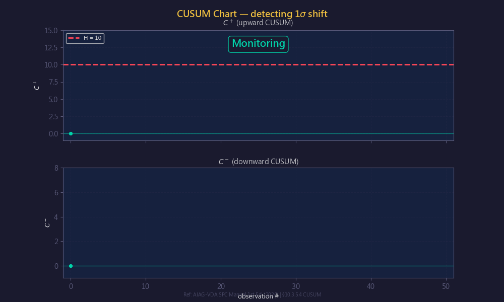
• Tabular CUSUM: C⁺ᵢ = max(0, C⁺ᵢ₋₁ + xᵢ − T − K); C⁻ᵢ = max(0, C⁻ᵢ₋₁ − xᵢ + T − K)
• K (reference value) = δ×σ/2, where δ is the target shift to be detected
• H (decision interval) = h×σ (h is typically taken as 4–5)
• The ARL₁ for detecting a 1σ shift ≈ 9.9 (§10.3.5.4, p.111 official ARL table), versus about 43.9 for the Shewhart chart — roughly 4.4× the sensitivity

Application scenarios: semiconductor process drift monitoring, pharmaceutical content deviation, tool wear trend detection.

Limitations: For large shifts (> 3σ) it is less intuitive than the Shewhart chart; it requires a preset target shift δ.

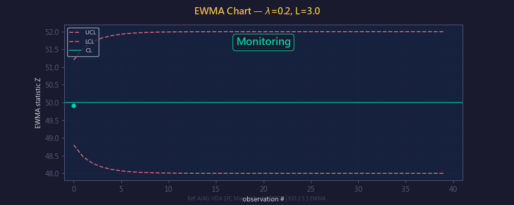
02 Exponentially Weighted Moving Average Control Chart (EWMA Chart)

It smooths short-term fluctuations through a weighted average to detect small shifts (AIAG & VDA, 2026, §10.3.5.5, p.116; see also ISO 7870-6).

• Recursive formula: Zᵢ = λxᵢ + (1−λ)Zᵢ₋₁
• Control limits: UCL/LCL = T ± L×σ√(λ/(2−λ)×[1−(1−λ)²ⁱ])
• Weighting coefficient λ (0 < λ ≤ 1) controls the influence of historical data: a small λ (0.05–0.1) detects small shifts; a large λ (0.2–0.4) approaches the behavior of the X̅ chart
• The control limits converge over time: wider at the start (less information), then trending toward fixed values once at steady state

EWMA vs CUSUM comparison:

Aspect	CUSUM	EWMA
Design requirement	Requires a preset target shift δ	No preset required; more flexible design
1σ shift ARL₁	≈ 9.9	≈ 10.3 (λ=0.1)
Non-normal data	More sensitive to the normality assumption	Performs well even for non-normal data (CLT effect)
Suitable scenarios	Best when the expected shift is known	Gradual chemical changes, measurement system drift tracking

03 Pre-Control Chart

A non-statistical control chart that simply divides the tolerance into zones based on the specification limits (AIAG & VDA, 2026, §10.3.2.7, p.90: “Control Charts for Preliminary Control”, a simple form of partitioning among tolerance-related charts).

• Green zone: specification center ± 1/4 of the specification width
• Yellow zone: from the green zone to the specification limit
• Red zone: beyond specification

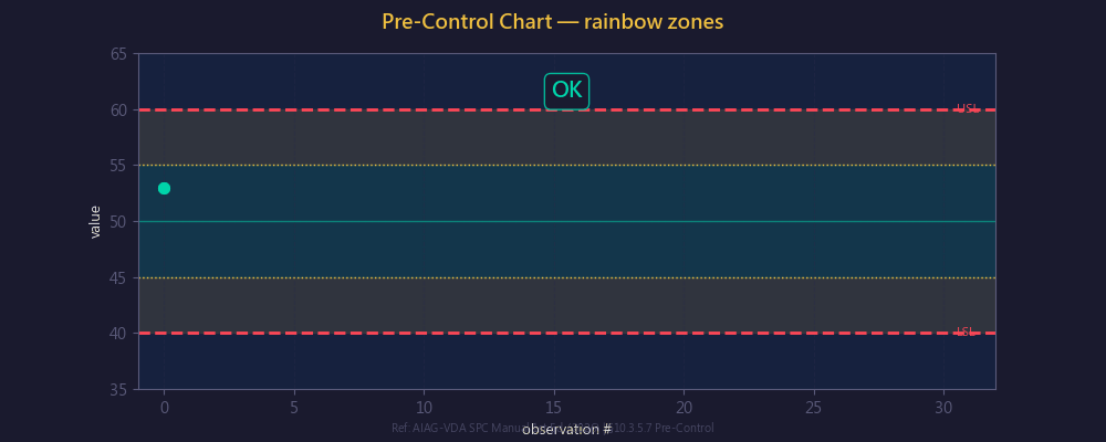
Decision rules:

• 5 consecutive points in the green zone → process passes
• 2 consecutive yellow points (same side) → adjust the machine
• Any red point → stop the machine

Advantages: No historical data required, simple setup, decision completed within 5 minutes. Theoretical basis: assuming Cpk ≥ 1.33, the probability of falling in the green zone is > 86%.

Application scenarios: first-article confirmation in mold trials, quick verification after line changeover, low-volume high-mix production environments.

Limitations: Cannot detect trends or cyclical patterns; does not provide a quantitative process capability index.

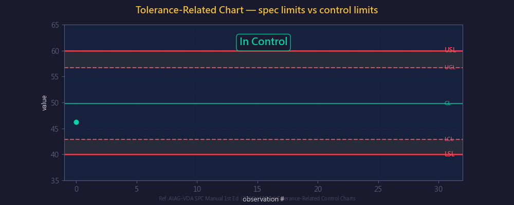
04 Tolerance-Related Control Chart

Control limits are set based on the specification limits (rather than process statistics) (AIAG & VDA, 2026, §10.3.4, p.104).

The Yellow Book §10.1 places two concepts side by side: Process-Related focuses on detecting process stability; Tolerance-Related focuses on confirming that the product is within specification.

It is suitable for scenarios where Cpk is very high and the control limits are relaxed to reduce the false alarm rate. The difference from the Shewhart control chart lies in the basis for setting the limits — the Shewhart chart uses the process ±3σ as its limits, while the tolerance-related chart references USL/LSL.

---

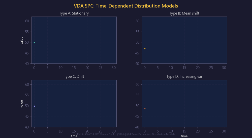
2. Time-Dependent Models

Three typical special-cause patterns generated by process data over time:

Pattern	Characteristics	Typical root cause	Trigger rule
Drift	Data continuously move in the same direction	Tool wear, chemical aging	WE Rule 3 (consecutively increasing/decreasing)
Cycle	Repetitive fluctuation	Day-night ambient temperature variation, shift effects	Regular alternation up and down
Shift	Sudden change in level	Material change, machine adjustment, operator change	WE Rule 2 (consecutively on the same side)

Autocorrelation problem: When data exhibit time dependence, the ±3σ assumption of traditional control charts is violated. Solutions: EWMA/CUSUM control charts, residual control charts, or eliminating the known time trend before charting.

---

3. Pearson Non-Normal Control Charts

Why are non-normal control charts needed?

When data do not follow a normal distribution, the traditional ±3σ control limits lead to high false-alarm or missed-detection rates. The new edition of the manual explicitly states in §10.3.5.2 (p.106): when the subgroup size n < 9 and the data are clearly non-normal, the Pearson control chart should be the first choice.

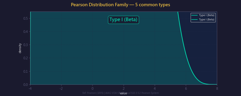
The Pearson Distribution System

This section of the Yellow Book uses estimates of skewness (γ₁) and kurtosis (β₃), and directs readers to refer to the ISO 22514-4 standard to define the standardized Pearson distribution classification and calculation formulas (AIAG & VDA, 2026, §10.3.5.2, p.106). The Pearson distribution system (Pearson family) classifies data into different skewed distributions based on skewness and kurtosis; the following are common classification mappings within the Pearson system:

Type	Corresponding distribution	Typical application
Type I	Beta distribution	Bounded data
Type III	Gamma / χ² distribution	Casting wall thickness (right-skewed)
Type IV–VI	Various asymmetric distributions	Complex skewed data
Type VII	Student-t family distribution	Symmetric heavy-tailed data

Note: The detailed classification definitions of Type I–VII come from the statistical literature of the Pearson distribution system (Pearson, 1895) and the ISO 22514-4 standard. The Yellow Book itself refers to it collectively as the “Pearson family” and does not list out the name of each type individually.

Control Limit Calculation

Use exact quantiles to replace the traditional ±3σ:

• LCL = F⁻¹(0.00135) — the 0.135% quantile of the distribution
• UCL = F⁻¹(0.99865) — the 99.865% quantile of the distribution
• Equivalent to the ±3σ coverage (99.73%) under a normal distribution, but the limits are asymmetric

Why not use a Box-Cox transformation?

Although mathematical transformations such as Box-Cox can convert skewed data into approximately normal data, they have a fatal practical problem on the shop floor:

“only be used as SPC control charts on site to a limited extent”
— AIAG & VDA (2026), §10.3.2.6, on the on-site practical limitations of transformed control charts

The reason: a transformed control chart requires an “inverse transformation” to return to the original physical units, which is difficult for shop-floor operators to interpret. The Pearson control chart, by contrast, directly uses the original data units to establish asymmetric limits, greatly improving on-site intuitiveness.

---

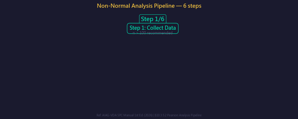
4. Non-Normal Distribution Analysis Pipeline

A 6-step end-to-end workflow for the automated analysis pipeline:

Step	Action	Description
1	Data input	Compute sample statistics (n, x̄, s, γ₁, γ₂)
2	Normality test	Shapiro-Wilk (n < 5000) or Anderson-Darling; p < 0.05 indicates non-normal
3	Pearson classification	Compute β₁, β₂ → determine the distribution type (I–VII or Normal)
4	Distribution fitting	Fit parameters (shape, location, scale) based on the classification result, using maximum likelihood estimation
5	Quantile calculation	F⁻¹(0.00135) = LCL, F⁻¹(0.99865) = UCL
6	OOC determination	Compare data points with the non-normal control limits, combined with out-of-control rules

---

5. Intelligent Chart Selection Decision Engine

AIAG-VDA divides control chart application into the analysis chart phase (Analysis Chart) and the SPC chart phase (SPC Chart). The chart selection decision occurs in the analysis phase:

Scenario	Condition	Recommended approach
A — Normal	Normality test passes	Shewhart control chart (X̅-R/S or I-MR); ±3σ limits are effective
B — Skewed	n = 1 and data are non-normal	Pearson asymmetric control limits, to avoid false alarms caused by symmetric limits
C — Autocorrelated	Data are autocorrelated	EWMA / CUSUM memory-type control charts

Key concept: If the distribution shape changes during the SPC control chart period, this is itself a special-cause signal; the root cause should be investigated rather than switching the control chart. The X̅ control chart (n ≥ 4) is protected by the Central Limit Theorem — the subgroup averages approach normality — so in most cases non-normal control methods are not needed.

---

Frequently Asked Questions (Q&A)

Q1: Can CUSUM and EWMA be used at the same time?

Yes, but usually choosing one is sufficient. Both have similar capability for detecting small shifts (the 1σ shift ARL₁ is 9.9 and 10.3, respectively). CUSUM is suitable for scenarios where the expected shift is known; EWMA has a more flexible design and does not require a preset δ. In practice, the choice is mostly based on software support and engineer familiarity.

Q2: Can the Pre-Control chart replace the Shewhart control chart?

No. The Pre-Control chart is a quick screening tool based on the specification limits; it cannot detect patterns such as trends and cyclicality, nor does it provide a quantitative process capability index. It is suitable for quick verification in the early stage of a line changeover (decision within 5 minutes), or as a temporary solution in low-volume high-mix production when there is insufficient historical data to establish a formal control chart.

Q3: How do you determine whether data are autocorrelated?

Use an autocorrelation function (ACF) plot or the Durbin-Watson test. If there is a significant correlation between adjacent observations (ACF lag-1 significantly different from zero), the ±3σ assumption of the traditional Shewhart control chart is violated. In this case, EWMA/CUSUM should be used, or a control chart should be built on the residuals.

Q4: How much data does a Pearson control chart need for reliable classification?

At least 125 individual values (≥ 25 subgroups) are needed to reliably estimate skewness and kurtosis. Too few samples lead to unstable Pearson classification, especially for the determination of Type IV (which has no closed form). The analysis chart phase should collect sufficient data and complete the classification in one pass.

Q5: When should a Tolerance-Related control chart be used?

When the process Cpk is much greater than 1.33 (e.g., Cpk > 2.0), using ±3σ control limits leads to overly frequent false alarms (because the process variation is far smaller than the specification width). In this case, one can consider relaxing the control limits based on the specification limits to reduce unnecessary stoppage investigations. But note: this sacrifices some detection sensitivity.

---

References

1. AIAG & VDA (2026). Statistical Process Control SPC Manual, 1st Edition, §10.3.5 (Advanced Charts), §10.3.2.7 (Pre-Control), §10.3.4 (Tolerance-Related).
2. AIAG (2005). Statistical Process Control SPC Manual, 2nd Edition.
3. ISO 7870-6:2016. Control charts — Part 6: EWMA control charts.
4. Pearson, K. (1895). Contributions to the mathematical theory of evolution. II. Skew variation in homogeneous material. Philosophical Transactions of the Royal Society A, 186, 343-414.
5. Montgomery, D.C. (2019). Introduction to Statistical Quality Control, 8th Edition. Wiley.

This article was written by the quality technology team at MiDFUN, based on an analysis of the original text of the AIAG-VDA SPC Manual 1st Edition (2026).
The MiDFUN SPC system already has built-in advanced control chart features such as the Pearson non-normal control chart, CUSUM, and EWMA.
For SPC system implementation consultation, please contact us.